
Google BigQuery Adds AI-Powered Analytics Functions for Agent-Ready Data Investigation
Google Cloud has introduced six BigQuery augmented analytics TVFs that use AI, ML and statistical methods to automate tasks such as finding key drivers, detecting changes, measuring causal effects, identifying trends and analyzing seasonality.
Xcademia Team
Xcademia Research Team
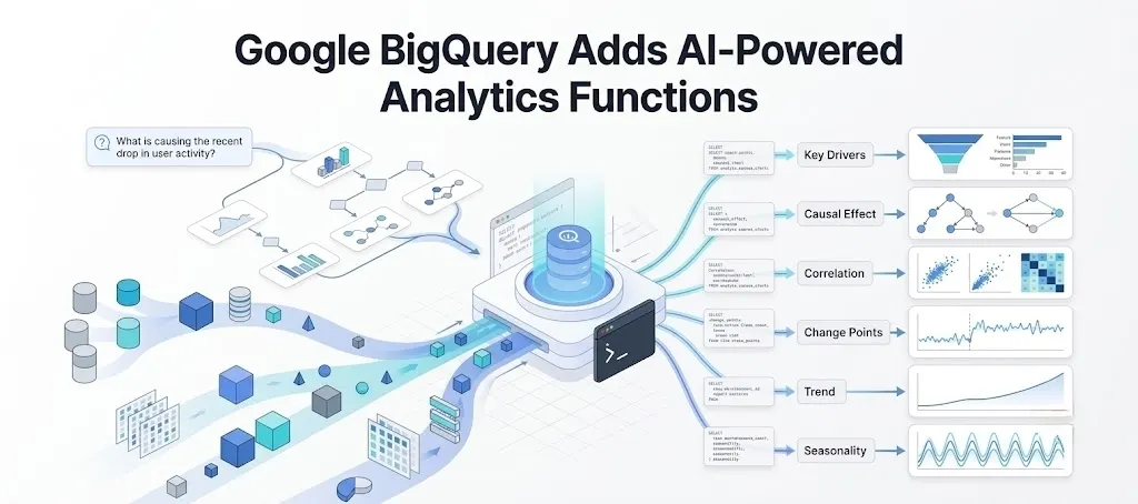
Google Cloud is expanding BigQuery's analytical capabilities with a new set of augmented analytics Table-Valued Functions (TVFs) designed to automate parts of complex data investigation.
The six new functions combine AI, machine learning and statistical methods to help users investigate questions such as why a metric changed, which factors contributed to that change, whether two metrics are related, and whether a business intervention produced an observable effect.
The functions run directly in BigQuery, where the data resides. Google Cloud says this can reduce the need to move data into external analytical tools.
The functions also produce structured SQL outputs. That makes them suitable for integration into AI agent skills and conversational analytical workflows.
The result is a model in which an AI agent can potentially move through multiple analytical steps instead of simply returning a single answer.
Six BigQuery Functions Target Different Analytical Questions
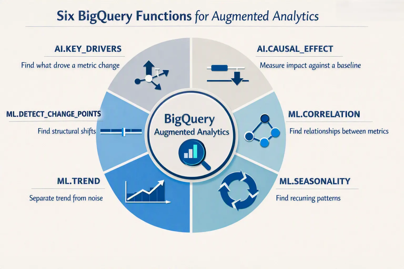
Google Cloud is introducing six augmented analytics functions, with each addressing a specific analytical problem.
1. AI.KEY_DRIVERS
Purpose: Identify the leading factors behind an increase or decrease in a metric between two time periods or groups.
Example question:
"Why did revenue spike this quarter compared to last quarter?"
The function can examine multiple dimensions and identify segments that contribute to a metric difference.
2. AI.CAUSAL_EFFECT
Purpose: Estimate the impact of an action or event by comparing observed results with an expected baseline.
Example question:
"How much of the revenue lift came from our pricing update rather than organic growth?"
The source demonstrates this using a counterfactual approach based on ARIMA_PLUS.
3. ML.CORRELATION
Purpose: Evaluate the direction and strength of relationships between pairs of numeric metrics.
Example question:
"Does increased user session duration correlate with higher lifetime customer value?"
This function focuses on relationships between numerical measures rather than directly establishing causation.
4. ML.DETECT_CHANGE_POINTS
Purpose: Identify dates or intervals where a metric experiences a structural shift compared with surrounding patterns.
Example question:
"When did platform latency experience persistent structural changes?"
This can be particularly useful for identifying when something changed before investigating why it changed.
5. ML.TREND
Purpose: Separate underlying growth or decline from short-term fluctuations and noise.
Example question:
"What is the underlying trend in revenue over the past year?"
The function is designed to help analysts distinguish longer-term movement from temporary spikes and drops.
6. ML.SEASONALITY
Purpose: Identify recurring patterns across hours, days, weeks, months or quarters.
Example question:
"Which days of the week consistently experience the highest server load?"
This can help identify recurring cycles within time-series data.
The Important Part: These Functions Can Be Chained
Google Cloud's announcement goes beyond presenting six separate functions.
A central part of the demonstration is that the functions can be chained together.
The output from one analytical function can become the input for the next stage of investigation.
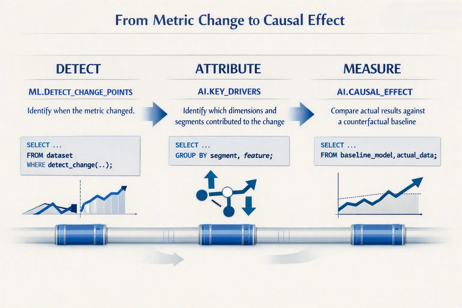
For example, a team might first identify when a metric changed, then investigate what drove the change, and finally estimate how much of the observed change was actually caused by a particular intervention.
The source demonstrates this workflow using three functions:
ML.DETECT_CHANGE_POINTS → AI.KEY_DRIVERS → AI.CAUSAL_EFFECT
This turns the analysis into a sequence rather than a single query.
How the SQL Workflow Works
The Austin Bikeshare example in the announcement provides a concrete demonstration of the workflow.
Google Cloud uses the public dataset:
bigquery-public-data.austin_bikeshare.bikeshare_tripsThe analysis starts with daily trip counts.
A SQL query uses TIMESTAMP_TRUNC() to group trip timestamps by day and COUNT(*) to calculate the number of trips.
The resulting daily dataset is then passed into:
ML.DETECT_CHANGE_POINTSThe function receives the metric column and timestamp column and returns information about detected changes, including the beginning and end of the identified intervals and statistical information about the affected period.
This first step answers:
When did the underlying pattern change?
Step 1: Detecting the Change
The source's first analytical stage uses ML.DETECT_CHANGE_POINTS against daily trip volumes.
The SQL workflow essentially follows this structure:
WITH daily_trips AS (
  SELECT
    TIMESTAMP_TRUNC(start_time, DAY) AS trip_day,
    COUNT(*) AS total_trips
  FROM `bigquery-public-data.austin_bikeshare.bikeshare_trips`
  GROUP BY 1
)
SELECT
  begin_timestamp,
  end_timestamp,
  metrics.avg AS avg_daily_trips,
  metrics.min AS min_daily_trips,
  metrics.max AS max_daily_trips,
  metrics.count AS duration_days
FROM ML.DETECT_CHANGE_POINTS(
  (SELECT * FROM daily_trips),
  data_col => 'total_trips',
  timestamp_col => 'trip_day'
);
The important point is not simply the function call.
The query first creates an analytical time series. The TVF then examines that series to identify structural shifts.
Google Cloud's example identifies a February 2018 change point in the Austin Bikeshare data.
The source connects this period with the Austin City Council's Dockless Mobility Pilot Program and a promotional University of Texas membership initiative described later in the analysis.
Step 2: Finding What Drove the Change
Knowing when something changed is only the beginning.
The next question is:
What caused the metric to move?
For this stage, the source uses AI.KEY_DRIVERS.
The analysis creates a dataset containing dimensions such as:
start_station_nameend_station_namesubscriber_typebike_typetrip_count
It then separates the data into an interest group representing the period after the detected change and a reference group representing the period before it.
The function is called with the relevant dimensions and a top_k value to return the leading contributing segments.
A simplified representation of the SQL workflow is:
SELECT
  drivers,
  metric_interest,
  metric_reference,
  difference,
  relative_difference,
  unexpected_difference,
  contribution
FROM AI.KEY_DRIVERS(
  (SELECT * FROM daily_segments),
  metric_col => 'trip_count',
  interest_label_col => 'after_shift',
  dimension_cols => [
    'start_station_name',
    'end_station_name',
    'subscriber_type',
    'bike_type'
  ],
  top_k => 10
);
The output identifies combinations of dimension values that contributed to the observed change.In the source example, the analysis found that the increase was concentrated in particular membership and station segments.
Google Cloud reports that overall trip count increased by 374.7%, or 40,159 trips, between the reference and interest windows.
It also reports particularly large increases associated with U.T. Student Memberships and trips ending at the 21st & Speedway @PCL station.
The source connects these results with a University of Texas promotional partnership that offered free annual memberships to UT students.
Step 3: Measuring the Causal Effect
Finding a change and identifying contributing factors still does not necessarily tell an analyst how much of that change can be attributed to a particular intervention.
That is where the third stage comes in.
Google Cloud uses:
AI.CAUSAL_EFFECTThe function compares observed results with a counterfactual baseline.
In the Austin Bikeshare example, the analysis uses historical data leading up to the intervention and specifies the detected February 2018 breakpoint as the intervention timestamp.
The source explains that the function can construct an ARIMA_PLUS counterfactual to estimate what the metric would have looked like if the intervention had not occurred.
The SQL structure includes parameters such as:
SELECT
  *
FROM AI.CAUSAL_EFFECT(
  (SELECT * FROM daily_trips),
  data_col => 'total_trips',
  timestamp_col => 'trip_day',
  intervention_timestamp => '2018-02-11 00:00:00',
  output_time_series => TRUE
);
The result can be viewed as a time series comparing the observed metric with the predicted counterfactual.
Google Cloud also shows an option to set:
output_time_series => FALSEThis returns a summary of the estimated lift instead of the full time-series output.
According to the source, the analysis estimated a 358% volume surge above the organic baseline, corresponding to 89,775 incremental trips, with a 99.9% probability of causal effect.
These figures are results from Google's demonstration using the Austin Bikeshare public dataset and should not be interpreted as general performance benchmarks for the function.
BigQuery Functions Can Also Work With Conversational Analytics
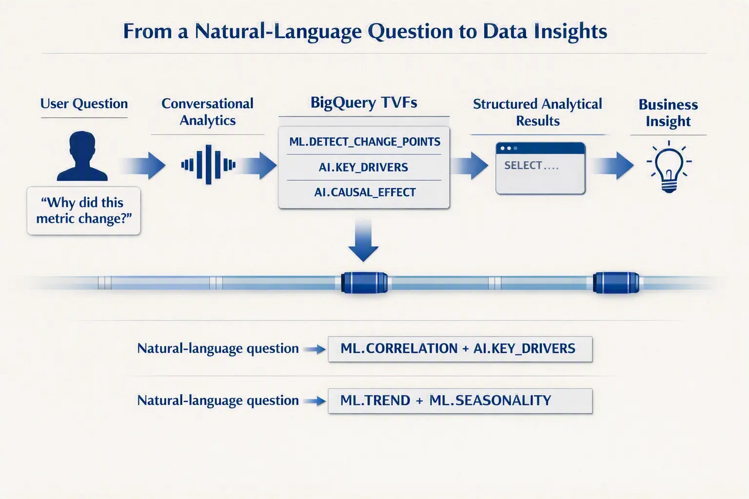
Google Cloud is also connecting these augmented analytics capabilities with Conversational Analytics.
Conversational Analytics allows users to interact with data through natural-language prompts.
The new BigQuery augmented analytics functions are now available through this workflow.
This means an analytical request can potentially involve multiple functions behind the scenes.
Instead of manually writing every analytical step, a user can ask a question in natural language and have the analytical workflow orchestrated across the relevant functions.
The source provides two examples.
Example 1: Chicago Taxi Trips
The first example uses the Chicago Taxi Trips public dataset.
The prompt asks:
"What metric has the strongest correlation with drivers getting tipped? Then run an attribution analysis to tell me which categorical dimensions most disproportionately drive that specific metric."
The workflow combines:
ML.CORRELATIONwith:
AI.KEY_DRIVERSThe first function evaluates relationships between numerical metrics.
The second then performs an attribution analysis to identify categorical dimensions associated with the selected metric.
The source reports that credit card payments were identified as a major positive driver of trip distance, while trips originating from O'Hare International Airport were another positive factor in the analyzed data.
Cash transactions appeared as a negative driver in the example.
These findings are specific to the demonstration dataset and analytical question used in Google's article.
Example 2: Iowa Liquor Dataset
The second Conversational Analytics example uses the Iowa liquor sales dataset.
The prompt asks the system to:
Find the historical trend for bottles sold
Describe yearly seasonality patterns
The workflow combines:
ML.TRENDwith:
ML.SEASONALITYAccording to the source, the analysis identified long-term growth in bottle sales, along with recurring seasonal patterns.
The example reports higher activity during periods including October, December, May and June, with lower sales around January and February.
Again, these are observations from the public dataset used in the demonstration, not general claims about consumer behavior.
Why the SQL Examples Matter
The code examples in Google's announcement are important because they show how the new capabilities fit into an existing BigQuery workflow.
The functions are not presented simply as standalone AI tools.
They are called directly from SQL and operate on structured data inside BigQuery.
For data teams, that means the analytical process demonstrated in the announcement follows a familiar pattern:
Prepare the data → call the analytical function → inspect structured output → feed the result into the next analysis.
The Austin Bikeshare example makes this particularly clear.
The first query creates daily trip totals.
The change-point function identifies a period of structural change.
That output is then used to define the relevant time window for the key-driver analysis.
The resulting breakpoint is subsequently used as the intervention timestamp for the causal-effect analysis.
In other words, the workflow is connected.
The result of one analytical operation helps define the next operation.
Making Analytical Skills Available to AI Agents
Google Cloud also emphasizes the connection between these TVFs and AI agents.
Because the functions are compact and return structured SQL outputs, Google says they can be integrated as skills for AI agents.
The company has made skills for these TVFs available through the Google Skills GitHub repository, including BigQuery AI/ML skills.
This creates another layer on top of the SQL functions.
A traditional analytics workflow might require an analyst to determine which statistical method to use, write the SQL, inspect the results, and decide what to run next.
An agent-based workflow can potentially orchestrate those steps based on a natural-language request.
For example, a request to investigate an unexpected revenue change could involve:
Detect the change → identify the drivers → estimate the causal effect.
The underlying analytical functions remain explicit, while the agent can coordinate how they are used.
Additional details about how these skills perform in production environments were not disclosed in the announcement.
BigQuery's Six Functions at a Glance
Function | Primary purpose | Example analytical question |
|---|---|---|
| Find factors behind metric changes | Why did revenue change? |
| Estimate impact against a baseline | How much impact came from an intervention? |
| Measure relationships between metrics | Which metrics are related? |
| Find structural shifts | When did the metric pattern change? |
| Identify underlying direction | What is the long-term trend? |
| Find recurring cycles | When does the metric repeatedly rise or fall? |
The key distinction is that these functions answer different analytical questions.
Correlation does not answer the same question as causal effect.
Trend analysis does not identify the specific factors behind a change.
Change-point detection identifies when something shifted, while key-driver analysis investigates what contributed to the shift.
The source's chaining example brings these separate capabilities together.
What This Means for Agent-Ready Analytics
The announcement highlights a broader industry shift toward making analytical operations usable by AI agents while keeping the underlying data and analytical logic within established data platforms.
For enterprises, this could mean a move from isolated natural-language queries toward more structured, multi-step investigations.
The significance is not simply that users can ask questions in natural language.
The more important development is the ability to connect analytical operations into a workflow.
A question such as "Why did revenue change?" can involve several distinct analytical tasks:
When did the change occur?
Which segments contributed to it?
What portion can be attributed to a specific event or intervention?
BigQuery's new TVFs provide separate functions for these tasks, while Conversational Analytics and AI agent skills provide mechanisms for orchestrating them.
The practical value will depend on the quality of the underlying data, the analytical context, and how organizations use the resulting workflows.
Google Cloud did not provide broader production performance benchmarks, enterprise adoption figures, or independent validation in this announcement.
The Bigger Picture
Google Cloud's BigQuery update brings AI, machine learning and statistical analysis closer to the SQL layer.
The six new TVFs cover several common analytical problems, from identifying trends and seasonal patterns to finding change points, correlations, key drivers and estimated causal effects.
More importantly, the source demonstrates that these functions can be chained.
The Austin Bikeshare example moves from detecting a structural change to identifying its leading contributors and then estimating the intervention's effect.
Conversational Analytics extends the concept by allowing natural-language requests to orchestrate combinations of these analytical capabilities.
For AI agents, the structured SQL outputs and dedicated skills provide a more explicit set of analytical operations that can be incorporated into data investigation workflows.
The development reflects growing demand for analytics systems that can do more than retrieve data.
They increasingly need to help users investigate what happened, understand why it happened, and quantify the effect where the analytical method supports that conclusion.
Google Cloud has made documentation available for all six functions, while the associated BigQuery AI/ML skills are available through Google's Skills GitHub repository.
Source: Google Cloud Blog
About the Author